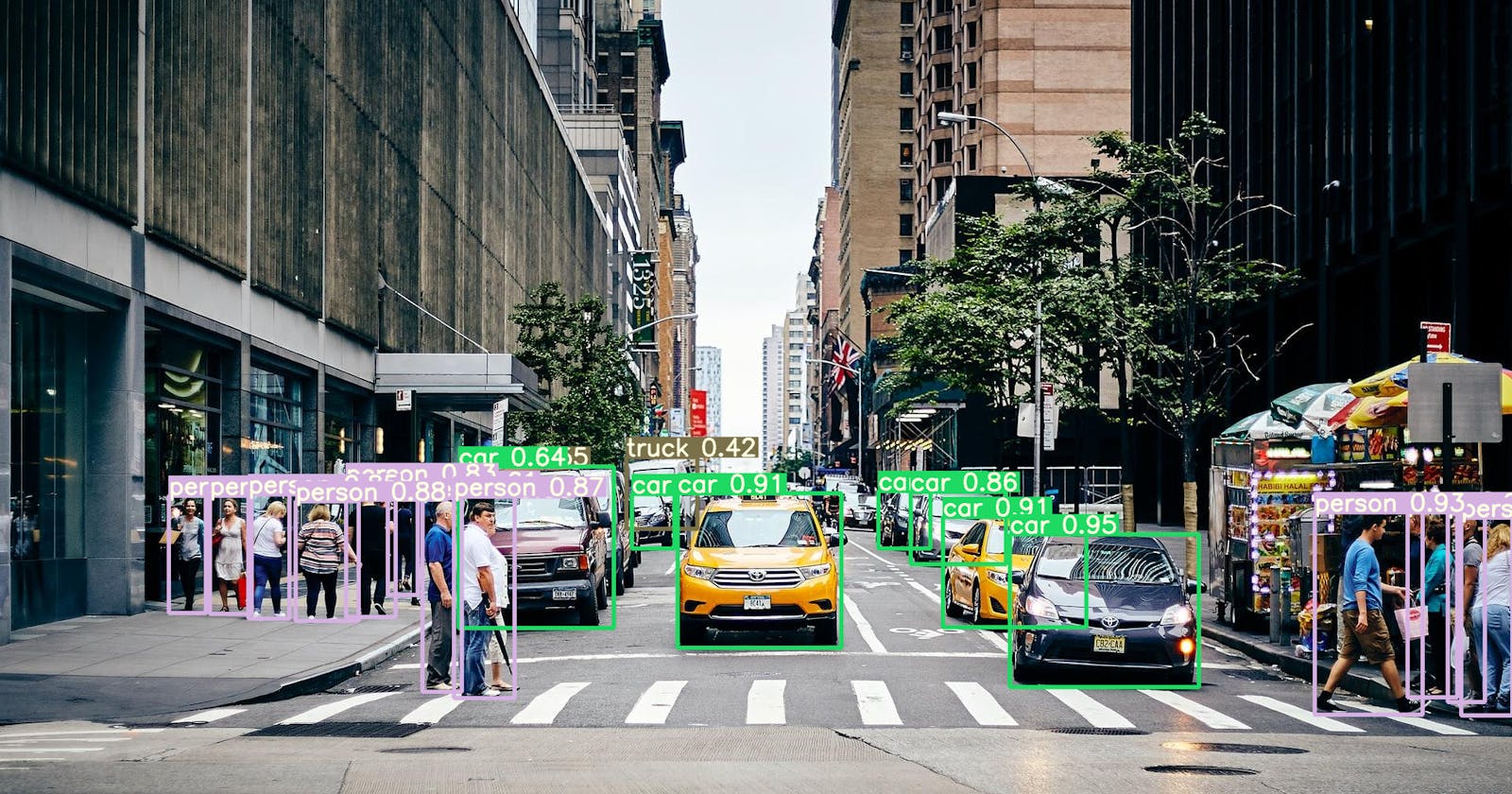
Getting Started with OpenCV: A Hands-on Guide(Part-1)
A Beginner's Guide to Computer Vision with OpenCV
Introduction:
OpenCV (Open Source Computer Vision) is a free and open-source library of computer vision and machine learning algorithms. It was originally developed by Intel and later supported by Willow Garage and Itseez. OpenCV has C++, Python, and Java interfaces, and it supports Windows, Linux, Mac OS, iOS, and Android.
OpenCV is widely used in a variety of applications, including security and surveillance, self-driving cars, robotics, and even in the entertainment industry for special effects. It has a number of pre-trained classifiers for faces, eyes, smiles, and other important features. It also has numerous modules for image processing, feature detection, and machine learning, making it a powerful tool for building intelligent systems.
In this blog, we will explore the various features and functions of OpenCV, and demonstrate how to use them to build practical applications in computer vision.
Installing libraries:
- we create a separate environment using Conda.
conda create --name compviz python=3.9
After creating Env, switch to that env by
conda activate compvizThen, install OpenCV using
pip, There are two options available in the PyPIpip install opencv-pythonpip install opencv-contrib-python
Option 1 will install the main package and Option 2 install the main package with extra/contributed packages. I will go with Option 2.
Let's start
After installing the libraries create a project file using mkdir opencvCourse and change the directory cd opencvCoursenow code . in that directory which will open VScode in the directory.
Reading Images and video
Reading Images
Create a file name read_images.pyand type these codes.
import cv2 as cv

img = cv.imread("./data/cat.jpg")
cv.imshow("Cat", img)

cv.waitKey(0)
In the above code first, we import the library, then in the first line we use OpenCV API
cv.read()to read the image file from the directory.Then, call
cv.imshow()with two arguments one is the name of the image frame and the image.And, at the last line, we call
cv.waitKey()the function which actually tells OpenCv how much time it will wait before destroying the window. and arguments0means it will wait an indefinite time until you press any key.
Now Reading Video
Same as above create a new file read_videos.py and type these codes. Don't worry I will explain it.
import cv2 as cv

# capture the video
cap = cv.VideoCapture("./data/penguins.mp4")

while True:
    isTrue, frame = cap.read()
    cv.imshow("Video", frame)

    if cv.waitKey(20) & 0xFF == ord('q'):
        break

cap.release()
cv.destroyAllWindows()
The line
cap = cv.VideoCapture("./data/penguins.mp4")is capturing or reading the video from the directory.The videos are actually moving frames of images, we are all somewhat familiar with the term FPS or (Frame per second). Here frame means the still image, so that means how many frames are moving or showing every second passing by.
we don't know how many frames or images are in that videos that's why we use a while loop to looping through every frame of the videos.
OpenCV read videos as a collection of frames with
isTrue, frame = cap.read()so we read those images withcap.read()and it has two values one isbooleanand the other is animageor frame.then, the next line as before
cv.imshow("Video", frame)Next, a condition for the video to run for 20 sec, and if you press the
'q'key then it stops immediately.After exiting from the
whileloopcapture functionrelease the video and OpenCV will destroy all the windows created during the run.
Now you know the basics of how to start with OpenCV.
Let's explore some basic functions of OpenCV
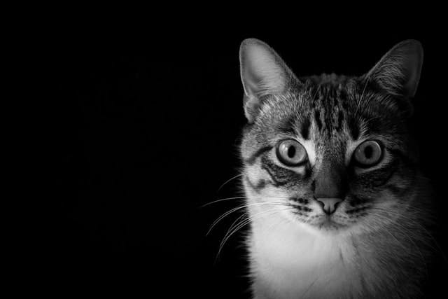
Converting to Gray Scale using
cv.cvtColor()function.import cv2 as cv img = cv.imread("./data/cat.jpg") cv.imshow("Cat", img) # Converting to gray image gray_cat = cv.cvtColor(img, cv.COLOR_BGR2GRAY) cv.imshow('Gray_Cat', gray_cat) cv.waitKey(0)
Blurring image with
cv.GaussianBlur()function. In that function, you have to provide a kernel for convolution which should positive and odd. here, Kernel is (7,7) as a Tuple.import cv2 as cv # Read in an image img = cv.imread('data/Photos/cat.jpg') # Blur blur_cat = cv.GaussianBlur(img, (7,7), cv.BORDER_DEFAULT) cv.imshow('Blur_cat', blur_cat) cv.waitKey(0)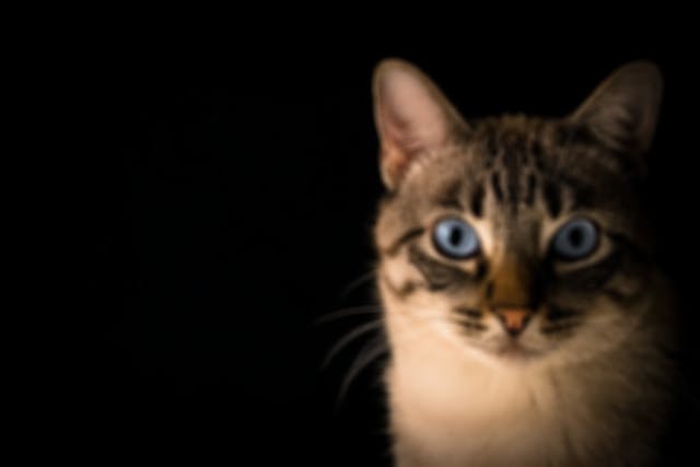
Edge Detection using
cv.canny()function. The first argument is the input image, second and third are minVal and maxVal respectively, there are more arguments such as aperture_size which is the Sobel kernel used to find image gradient. we will apply Canny after applying Blur, it works better than directly applying it to the original image.import cv2 as cv import matplotlib.pyplot as plt # Read in an image img = cv.imread('data/Photos/cat.jpg') # cv.imshow('Park', img) blur = cv.GaussianBlur(img, (7,7), cv.BORDER_DEFAULT) # Edge Cascade canny = cv.Canny(blur, 125, 175) # cv.imshow('Canny Edges', canny) plt.subplot(121),plt.imshow(img, cmap="gray") plt.title('Original Image'), plt.xticks([]), plt.yticks([]) plt.subplot(122),plt.imshow(canny, cmap="gray") plt.title('Edge Image'), plt.xticks([]), plt.yticks([]) plt.show()Applying the Canny Edge function on the Original Image.
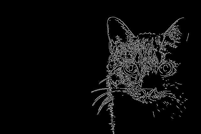
Applying the canny Edge function on the Blurred Image.
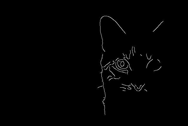
Do you see the difference between the images?
Blurred image get a better edge than the original.
Morphological Operations.
A set of operations that process images based on shapes.
The most basic morphological operations are: Erosion and Dilation
Removing noise.
Isolation of individual elements and joining disparate elements in an image.
Finding intensity bumps or holes in an image.
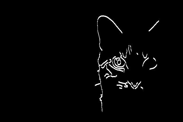
DILATION:
This operation consists of convolving an image with a kernel.
The kernel has a defined anchor point, usually the center of the kernel.
As the kernel is scanned over the image, we compute the maximal pixel value overlapped by the kernel and replace the image pixel in the anchor point position with that maximal value. As you can deduce, this maximizing operation causes bright regions within an image to "grow" (therefore the name dilation).
        import cv2 as cv

        # Read in an image
        img = cv.imread('data/Photos/cat.jpg')
        # cv.imshow('Park', img)

        blur = cv.GaussianBlur(img, (7,7), cv.BORDER_DEFAULT)
        # Edge Cascade
        canny = cv.Canny(blur, 125, 175)
        # Dilating the image
        dilated = cv.dilate(canny, (7,7), iterations=3)
        cv.imshow('Dilated', dilated)

        cv.waitKey(0)
EROSION:
This operation is the sister of dilation. It computes a local minimum over the area of a given kernel.
As the kernel is scanned over the image, we compute the minimal pixel value overlapped by the kernel and replace the image pixel under the anchor point with that minimal value.
Analogously to the example for dilation, we can apply the erosion operator to the original image. You can see in the result below that the bright areas of the image get thinner, whereas the dark zones get bigger.
  import cv2 as cv

  # Read in an image
  img = cv.imread('data/Photos/cat.jpg')

  blur = cv.GaussianBlur(img, (7,7), cv.BORDER_DEFAULT)
  # Edge Cascade
  canny = cv.Canny(blur, 125, 175)
  # Dilating the image
  dilated = cv.dilate(canny, (7,7), iterations=3)

  # Eroding
  eroded = cv.erode(dilated, (7,7), iterations=3)
  cv.imshow('Eroded', eroded)

  cv.waitKey(0)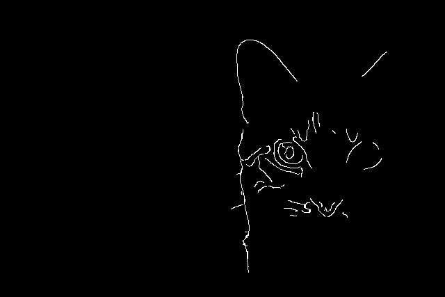
Resize the Image
```python import cv2 as cv import matplotlib.pyplot as plt
Read in an image
img = cv.imread('data/Photos/cat.jpg')
Resize
resized = cv.resize(img, (500,500), interpolation=cv.INTER_CUBIC) cv.imshow('Resized', resized)
cv.waitKey(0) ```

Now, you can see that the original image is resized to 500 by 500 pixels.
Conclusion
In this article, we learn some of the main functions to manipulate images and extract features from them. And also how to run a video using OpenCV. OpenCV is a vast library, which takes time to master, today you will take a little step toward it. Thank you for reading.
If you like my article, please share it with your audience. Comment your views.

